A PyTorch implementation of the Diffusion Transformer (DiT) model. With OpenAI’s Sora demonstrating the power of DiTs for multidimensional tasks, they represents a stable and efficient approach any diffusion task (vision, audio, robotics etc..). This implementation provides a clean, modular codebase to extend DiT for various generative applications.
Architecture
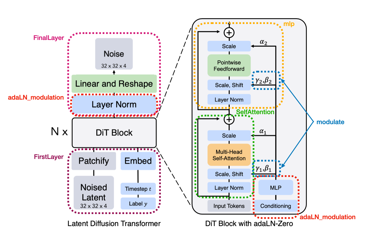
Implementation details
- Firstlayer: A Python class that initializes the input processing. It includes a
Patchifymodule to convert images into patches, a learnable positional embedding, and separate embedding layers for timesteps and class labels. The forward method combines these elements to prepare the input for the DiT blocks.b, c, h, w = x.shape p = self.patch_size # Reshape and permute to get patches x = x.reshape(b, c, h // p, p, w // p, p) x = x.permute(0, 2, 4, 3, 5, 1).contiguous() x = x.view(b, -1, p * p * c) # Project patches to embedding dimension x = projection(x) - LayerNorm: The LayerNorm affine transformation (scaling and shifting) is provided by a
adaLN_modulationmodule, which computes these parameters based on the conditioning vector. This allows the scaling and shifting to be input-dependent rather than fixed learnable parameters.self.adaLN_modulation = nn.Sequential( nn.SiLU(), nn.Linear(config.n_embd, 6 * config.n_embd, bias=True)) - MLP: Transformers struggle with spatial coherence in image tasks, often producing “patchy” outputs. To address this, we add a depth-wise convolution to the FFN layer, as introduced in the LocalViT paper. This allows the model to mix information from nearby pixels efficiently, improving spatial awareness and output quality with minimal computational cost.
- Modulate: Performs element-wise modulation of normalized inputs using computed shift and scale parameters. It’s used in both DiTBlock and FinalLayer to apply adaptive normalization.
shift, scale = self.adaLN_modulation(c).chunk(6, dim=1) x = modulate(self.norm_final(x), shift, scale) - SelfAttention: Multi-head self-attention module. It uses linear layers to project inputs into query, key, and value representations, applies scaled dot-product attention using PyTorch’s functional API, and projects the output back to the original embedding dimension.
- FinalLayer: It uses a LayerNorm without affine parameters, computes adaptive normalization parameters via the
adaLN_modulationmodule, and applies a final linear projection to reshape the output to the desired dimensions.
Classifier-free guidance
The official implementation uses classifier-free guidance improve the sample quality by combining conditional and unconditional generation. It modifies the denoising process to:
\[ \hat{\varepsilon}_\theta(x_t, c) = \varepsilon_\theta(x_t, \emptyset) + s \cdot (\varepsilon_\theta(x_t, c) - \varepsilon_\theta(x_t, \emptyset))\]Where $c$ is the condition, $\emptyset$ is a null condition, and $s > 1$ is the guidance scale.
While effective, this technique doubles computational cost. Our DiT implementation omits it, prioritizing computational efficiency for future robotics applications where real-time performance is crucial. By optimizing only $p_\theta(x_{t-1}|x_t,c)$, we balance generation quality with speed, better suiting time-sensitive robotic control tasks for example.
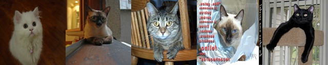
Dataset
To test the architecture, the DiT was trained on the Cat datasets which contains 20k high-res images of cats. Only the uncontinioned diffusion can be tested because all samples are cats.
A simple formatting is applied to every images:
torchvision.transforms.Compose([
    transforms.Resize((size, size)),
    transforms.RandomHorizontalFlip(),
    transforms.ToTensor(),
    transforms.Normalize([0.5], [0.5]),])
Variational Autoencoder
the DiT is trained in a reduced 32x32x4 latent space to lighten the calculations. Each images is projected on the latent space using a the Stable Diffusion VAE:
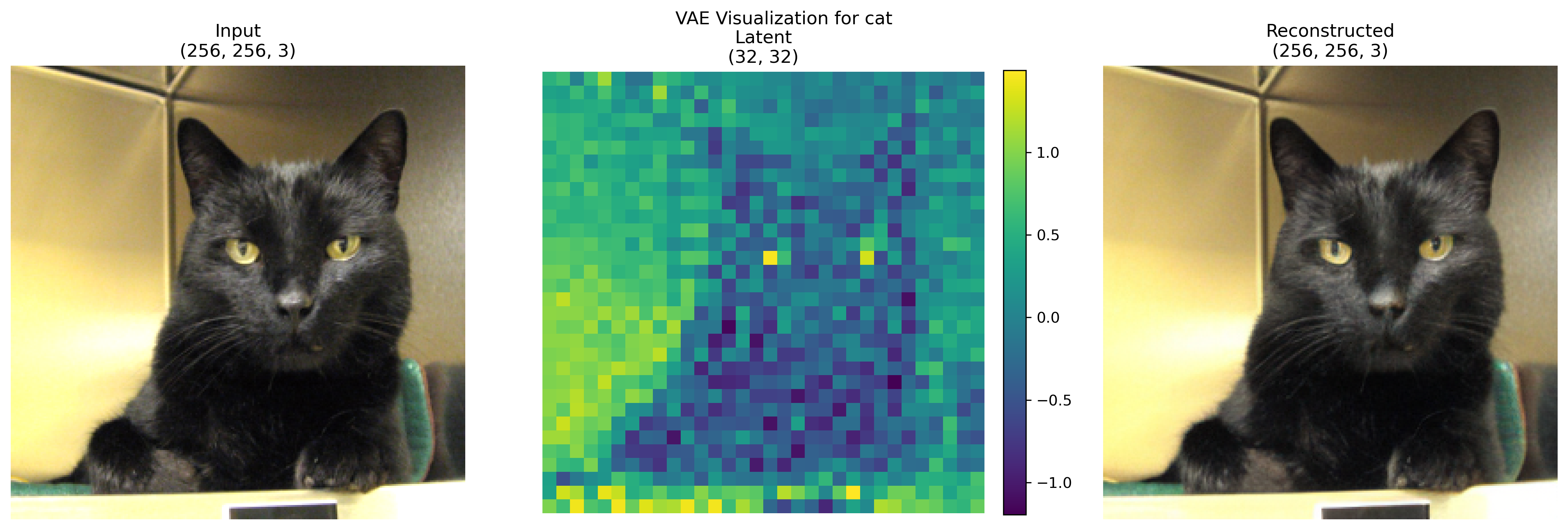
The Stable Diffusion VAE employs a crucial scaling factor of 0.18215, a legacy of its original training. This factor scales the latent representations during encoding (multiplication) and decoding (division), ensuring the latent space statistics match what the diffusion model expects. This scaling is essential for maintaining compatibility with pre-trained Stable Diffusion components and for achieving stable training and high-quality generation in DiT models.
class StableDiffusionVAE:
    def __init__(self, model_path="stabilityai/sd-vae-ft-mse"):
        self.scaling_factor = 0.18215
    [...]
    def encode(self, image):
        with torch.no_grad():
            latent = self.vae.encode(image).latent_dist.sample()
            latent = latent * self.scaling_factor
        return latent

    def decode(self, latent):
        latent = latent / self.scaling_factor
        with torch.no_grad():
            image = self.vae.decode(latent).sample
        return image
Simplified Diffusion Model Formulation
We implement a variance-preserving diffusion model using the DDPMScheduler from the Hugging Face Diffusers library, with the squaredcos_cap_v2 beta schedule. This approach maintains the Gaussian nature of the diffusion process while leveraging optimized scheduling for improved performance.
Noise Schedule
We use the squaredcos_cap_v2 beta schedule, which defines $\beta_t$ as:
where $T$ is the total number of timesteps and $s$ is a small constant (default 0.008). This schedule provides a smooth progression of noise levels, starting slow, accelerating in the middle, and then slowing down again at the end. The min operation caps the maximum beta value to 0.999.
Forward Process
The forward noising process remains unchanged:
\[ q(x_t|x_0) = \mathcal{N}(x_t; \sqrt{\bar{\alpha}_t} x_0, (1 - \bar{\alpha}_t)\mathbf{I}) \]$x_t$ can be sampled as:
\[ x_t = \sqrt{\bar{\alpha}_t} x_0 + \sqrt{1 - \bar{\alpha}_t} \varepsilon_{t}, \text{ where } \varepsilon_{t} \sim \mathcal{N}(0, \mathbf{I}) \]Here, $\bar{\alpha_{t}} = \prod_{s=1}^{t} (1 - \beta_s)$ is the cumulative product of noise scale factors, computed by the DDPMScheduler based on the beta schedule.
Reverse Process
The reverse process is used when generating and image. We directly predict the noise $\varepsilon_\theta$:
\[ p_\theta(x_{t-1}|x_t) = \mathcal{N}(x_{t-1}; \mu_\theta(x_t, t), \sigma_t^2 \mathbf{I}) \]Where:
\[ \mu_\theta(x_t, t) = \frac{1}{\sqrt{\alpha_t}}(x_t - \frac{\beta_t}{\sqrt{1-\bar{\alpha}t}}\varepsilon_{\theta(x_t, t)}) \]The DDPMScheduler handles the computation of $\alpha_t$, $\beta_t$, and $\bar{\alpha}_t$ based on the squaredcos_cap_v2 schedule, ensuring consistency between the forward and reverse processes.
Training Objective
We use the simplified loss:
\[ \mathcal{L_{\text{simple}}}(\theta) = |\varepsilon_{\theta(x_t, t)} - \varepsilon_{t}|^2 \]Implementation with HF’s DDPMScheduler
In practice, using the DDPMScheduler simplifies our implementation:
Initialization:
from diffusers import DDPMScheduler
scheduler = DDPMScheduler(num_train_timesteps=1000, beta_schedule="squaredcos_cap_v2")
Forward Process: The scheduler handles noise addition:
noisy_samples, noise = scheduler.add_noise(original_samples, noise, timesteps)Reverse Process: The scheduler computes the denoised sample given the model’s noise prediction:
denoised = scheduler.step(model_output, timestep, noisy_samples).prev_sample
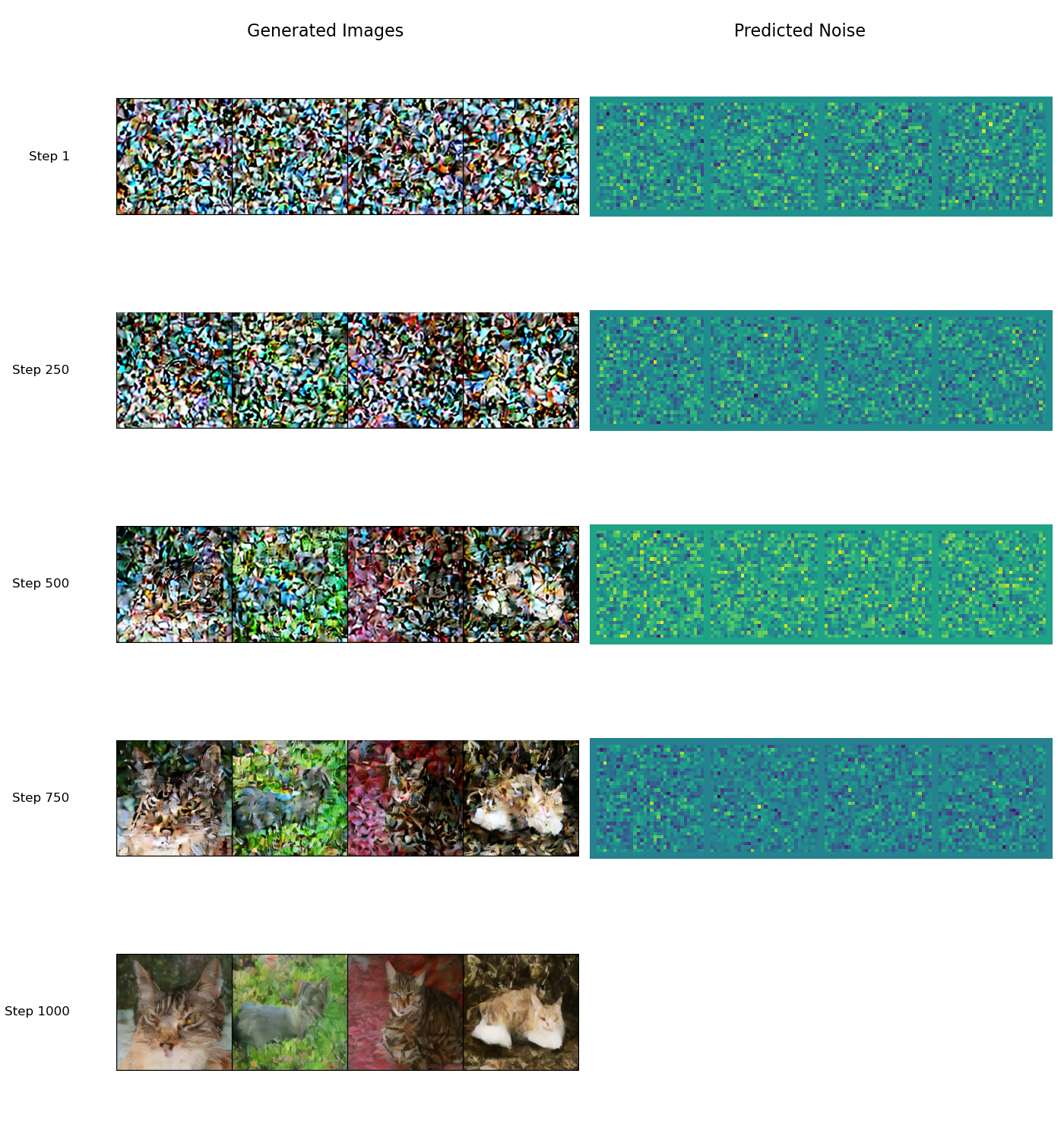
Results
The model was trained for for 22h a Nvidia A10 with the following hyperparameters:
- Patch size: 2
- Number of DiT blocks: 12
- Number of head: 12
- Embedding size: 768
- Batch size: 64
- Learning rate: 1e-4
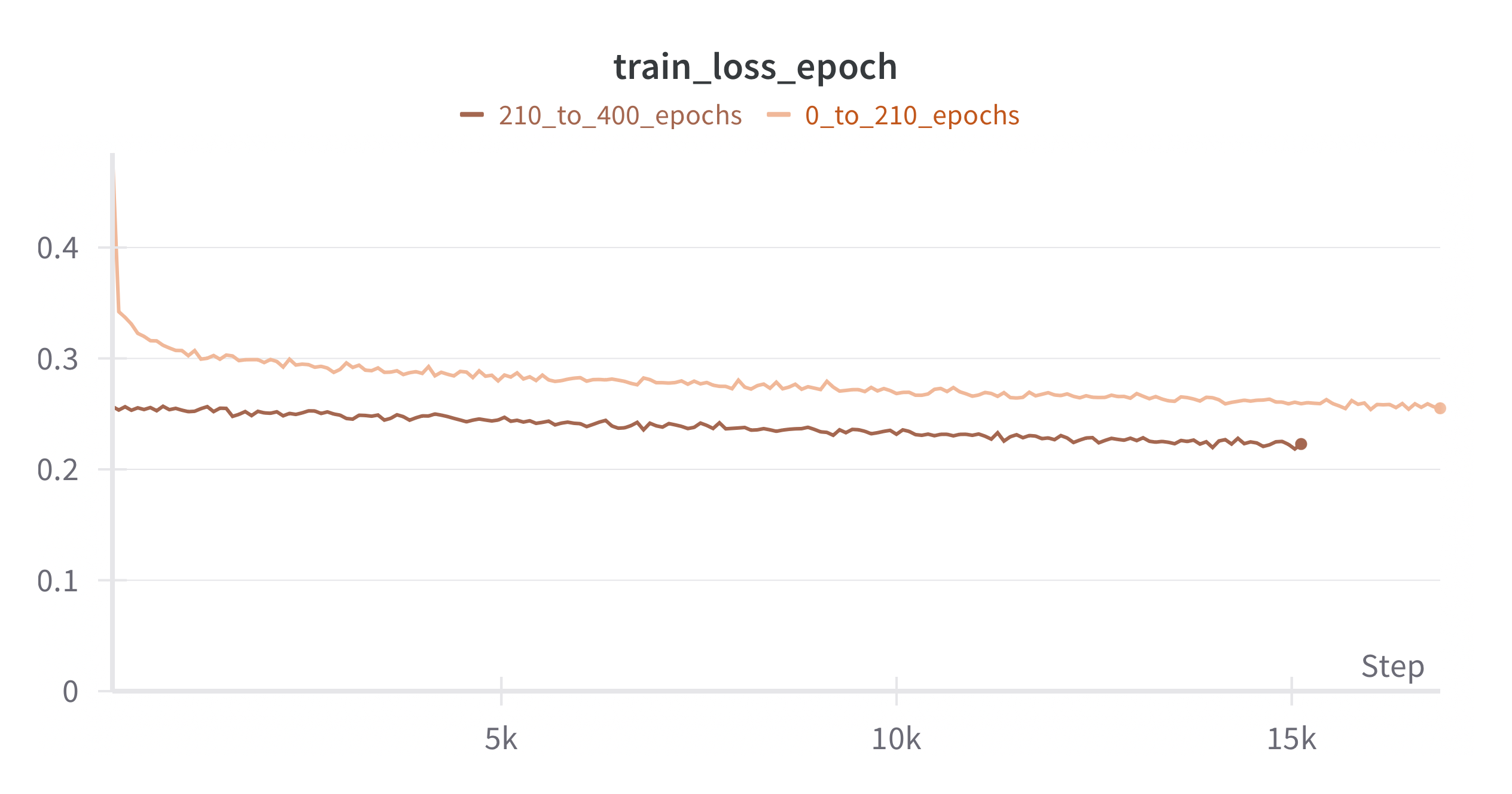
When stopped the model was still learning and its performances can stilll be improved by scalling its size and letting it learn longer. Here is a sampling example: